Stretched Mesh

The Particle In Cell example posted previously was based on a uniform, Cartesian mesh. Such meshes are common in PIC simulations for a good reason. The PIC method requires interpolation of properties between particles and the mesh. As such, it is important to be able to quickly find the containing cell and compute the interpolation factors. This is a non-trivial task on unstructured meshes. On the other hand, in the PIC method we also desire the cell sizes to scale inversely with the plasma density. Small cells are needed in dense regions to resolve the Debye length and larger cells are desired in the low density region to assure enough particles to reduce statistical noise. This is impossible with the uniform Cartesian mesh. Lucky for us, there exists another possibility: a stretched mesh. In this article, we’ll derive the governing equations and we’ll see how to implement a stretched mesh in PIC simulations.

Equations

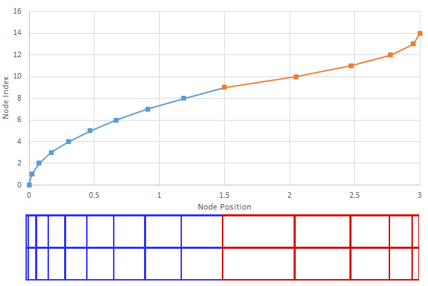
A stretched mesh is a mesh in which the cell spacing changes according to some analytical relationship. In this example we consider probably the simplest method in which the cell size increases linearly. This will result in a quadratic relationship for node positions. Cell spacing, as a function of the node index i can be written as
$$\Delta x =\Delta x_0 (1+ki)$$
where $k$ is the stretch factor and $i$ is assumed to be an integer in range $[0,n-1]$. Next, we need an expression for the node position. It is given by
$$x = \Delta x_0\left[i+0.5k(i^2-i)\right]+x_0$$
You will notice that this expression is the integral of the cell spacing evaluated at the half-way point. This is due to the fact that the the integral is continuous while our mesh-spacing is defined as a step-wise function. Also note that if $k=0$, we recover the uniform Cartesian mesh.

Node Index

The expression for node position can be inverted to obtain the relationship for node index. It requires solving the quadratic equation,
$$i = \frac{-b + \sqrt{b^2-4ac}}{2a}$$
with
$$\begin{align} a &= k \\ b &=2-k \\ c &= 2(x_0-x)/\Delta x_0 \end{align}$$

Stretch Factor

So far, we have not addressed the stretching factor. The stretch factor can be determined analytically given the following three user inputs: span of the mesh, reference cell size, and number of cells. It is computed by evaluating node position at the index of the last node, $c=n-1$
$$k= \frac{2\left[(x_{max}-x_0)/\Delta x_0 -c\right]}{c^2-c}$$

Shrinking Mesh

The opposite of a stretched mesh is a shrinking mesh. In the formulation below, $\Delta x_0$ is the size of the last (and smallest) cell. In other words, the cells shrink from some unknown size in the first cell to the user-defined value at the end.
$$\begin{align} \Delta x &= \Delta x_0 \left[1+k(n-2-i)\right]\\ x &= \Delta x_0\left[i+k\left(i(n-1.5)-0.5i^2\right)\right] + x_0 \end{align}$$

The coefficients for the quadratic equation for the node index on a shrinking mesh are:
$$\begin{align} a &= -k \\ b &=2[1+k(n-1.5)] \\ c &= 2(x_0-x)/\Delta x_0 \end{align}$$

Non-Uniform Mesh Finite Difference

First Derivative

The stretched mesh results in a non-uniform cell spacing, which will require adjustments to our finite difference formulation. Noticing that the central difference for the first derivative is basically the average of the slopes on the “plus” and “minus” sides of a node, we can write
$$\left(\frac{\partial \phi}{\partial x}\right)_i \approx \frac{1}{2}\frac{1}{\Delta x^+\Delta x^-} \Big[ \Delta x^- \phi_{i+1} + (\Delta x^+ – \Delta x^-)\phi_i – \Delta x^+\phi_{i-1}\Big]$$
where $\Delta x^- \equiv x_i-x_{i-1}$ and $\Delta x^+ \equiv x_{i+1}-x_i$. The standard central difference $(\phi_{i+1}-\phi_{i-1})/(2\Delta x)$ is recovered if $\Delta x^+=\Delta x^-$.

Second Derivative

Probably the most direct way to compute the non-uniform form for the second derivative (Laplacian) is to start with the Taylor series. We have
$$\begin{align} \phi_{i+1}&=\phi_i + \Delta x^+ \frac{\partial \phi}{\partial x} + \frac{\Delta^2x^+}{2}\frac{\partial^2\phi}{\partial^2 x}\\ \phi_{i-1}&=\phi_i – \Delta x^- \frac{\partial \phi}{\partial x} + \frac{\Delta^2x^-}{2}\frac{\partial^2\phi}{\partial^2 x} \end{align}$$
Next we mulitply the first equation by $\Delta x^-$ and the second by $\Delta x^+$. We can then add the two equations to eliminate the first derivative and obtain the following expression for the second derivative
$$\left(\frac{\partial^2\phi}{\partial x^2}\right)_i \approx \left[\frac{2}{\Delta x^-\Delta^2x^+ + \Delta x^+\Delta^2x^-}\right] \Big[\Delta x^-\left(\phi_{i+1}-\phi_i\right) + \Delta x^+\left(\phi_{i-1}-\phi_i\right)\Big]$$

Again, if mesh spacing is uniform, we recover the standard central difference for the second derivative $(\phi_{i+1}-2\phi_i+\phi_{i-1})/\Delta^2x$.

Multiple Zones

Stretched mesh is best utilized as a part of a complex mesh definition consisting of multiple zones. For instance, your domain may be best described by a shrinking mesh, followed by a uniform cell section, and then a growing mesh. The above relationship for computing the node index is valid only within each zone. Your code will first need to determine which zone the particle belongs to, and then computing the local node index. Finally, zone starting index is added to get the index in the global mesh.